v1.1.11

Overview

Updates:

New: Added dual-factor coloring support for binary dataset visualization.
Fix: Fixed legend order issues in DATASET_COLORSTRIP, DATASET_SYMBOL, and DATASET_DOMAINS functions.

1. Dual-Factor Coloring for Binary Dataset

Added support for dual-factor coloring in binary dataset visualization, allowing users to create more informative and visually appealing visualizations.

Data Preparation

# Set working directory for output files
setwd("~/Downloads/")

# Load required libraries
library(itol.toolkit)    # Main package for iTOL visualization
library(dplyr)           # Data manipulation and transformation
library(data.table)      # Fast file reading and data operations
library(ape)             # Phylogenetic tree operations
library(stringr)         # String manipulation utilities
library(tidyr)           # Data tidying and reshaping

# Load example data files
tree_1 <- system.file("extdata", "dataset4/otus.contree", package = "itol.toolkit")
data_file_1 <- system.file("extdata", "dataset4/annotation.txt", package = "itol.toolkit")
data_file_2 <- system.file("extdata", "dataset4/otutab_high.mean", package = "itol.toolkit")

# Read data files
data_1 <- data.table::fread(data_file_1)
data_2 <- data.table::fread(data_file_2)

Domain Visualization

Demonstrate the existing domain annotation feature that supports dual-factor coloring:

set.seed(123)  # Set random seed for reproducible results

# Create domain annotation unit with dual-factor coloring support
unit_6 <- create_unit(
  data = data_1 %>% select(ID, Class, Family),
  key = "New_in_v1.1.8",
  type = "DATASET_DOMAINS",
  color = "wesanderson",
  shape = "TL",
  tree = tree_1
)

Binary Data Processing

# Function to generate fluctuating columns for demonstration
generate_fluctuation_columns <- function(df, base_col, num_cols, fluctuation_range) {
  set.seed(123)  # Ensure reproducible results
  
  for (i in 1:num_cols) {
    col_name <- paste0(base_col, "_", i)
    # Generate values with random fluctuation around the base column
    df[[col_name]] <- df[[base_col]] * (1 + runif(nrow(df), -fluctuation_range, fluctuation_range))
  }
  return(df)
}

# Prepare data for binary visualization
# Select relevant columns and generate multiple samples
data_3 <- data_1 %>% select(ID, Asia, North_America, South_America)

# Generate 20 columns for each region with ±15% fluctuation
data_3 <- generate_fluctuation_columns(data_3, "Asia", 20, 0.15)
data_3 <- generate_fluctuation_columns(data_3, "North_America", 20, 0.15)
data_3 <- generate_fluctuation_columns(data_3, "South_America", 20, 0.15)

# Round numeric values for cleaner visualization
data_3[, 2:ncol(data_3)] <- round(data_3[, 2:ncol(data_3)])

# Enhanced data transposition function
transpose_with_first_column_as_header <- function(dt) {
  # Input validation
  if (!is.data.table(dt)) {
    stop("Input must be a data.table object.")
  }
  
  # Extract first column values as new column names
  new_col_names <- dt[[1]]
  
  # Transpose the data (excluding the first column)
  transposed_dt <- transpose(dt[, -1, with = FALSE])
  
  # Set column names from the first column data
  setnames(transposed_dt, new_col_names)
  
  # Add original column names as a new "Sample" column
  transposed_dt[, "Sample" := names(dt)[-1]]
  
  # Reorder columns to put Sample column first
  setcolorder(transposed_dt, c("Sample", new_col_names))
  
  return(transposed_dt)
}

# Apply transposition and prepare for binary visualization
data_3_t <- transpose_with_first_column_as_header(data_3)

# Clean sample names and sort for better organization
data_3_t <- data_3_t %>% 
  mutate(group = stringr::str_remove(stringr::str_remove(Sample, "\\d+$"), "_$")) %>% 
  arrange(Sample)

Binary Unit Creation

Create a binary visualization unit with enhanced styling:

# Create binary dataset unit with improved parameters
unit_7 <- create_unit(
  data = data_3,
  key = "New_in_v1.1.11",
  type = "DATASET_BINARY",
  color = "wesanderson",
  tree = tree_1
)

# Customize symbol height for optimal visualization
unit_7@specific_themes$basic_plot$height_factor <- 0.4

Output Generation

Combine all units and generate the final output:

# Create hub object and combine all visualization units
hub_1 <- create_hub(tree_1)
hub_1 <- hub_1 + unit_6 + unit_7

# Write output files with tree data
write_hub(hub_1, "~/Downloads/", with_tree = TRUE)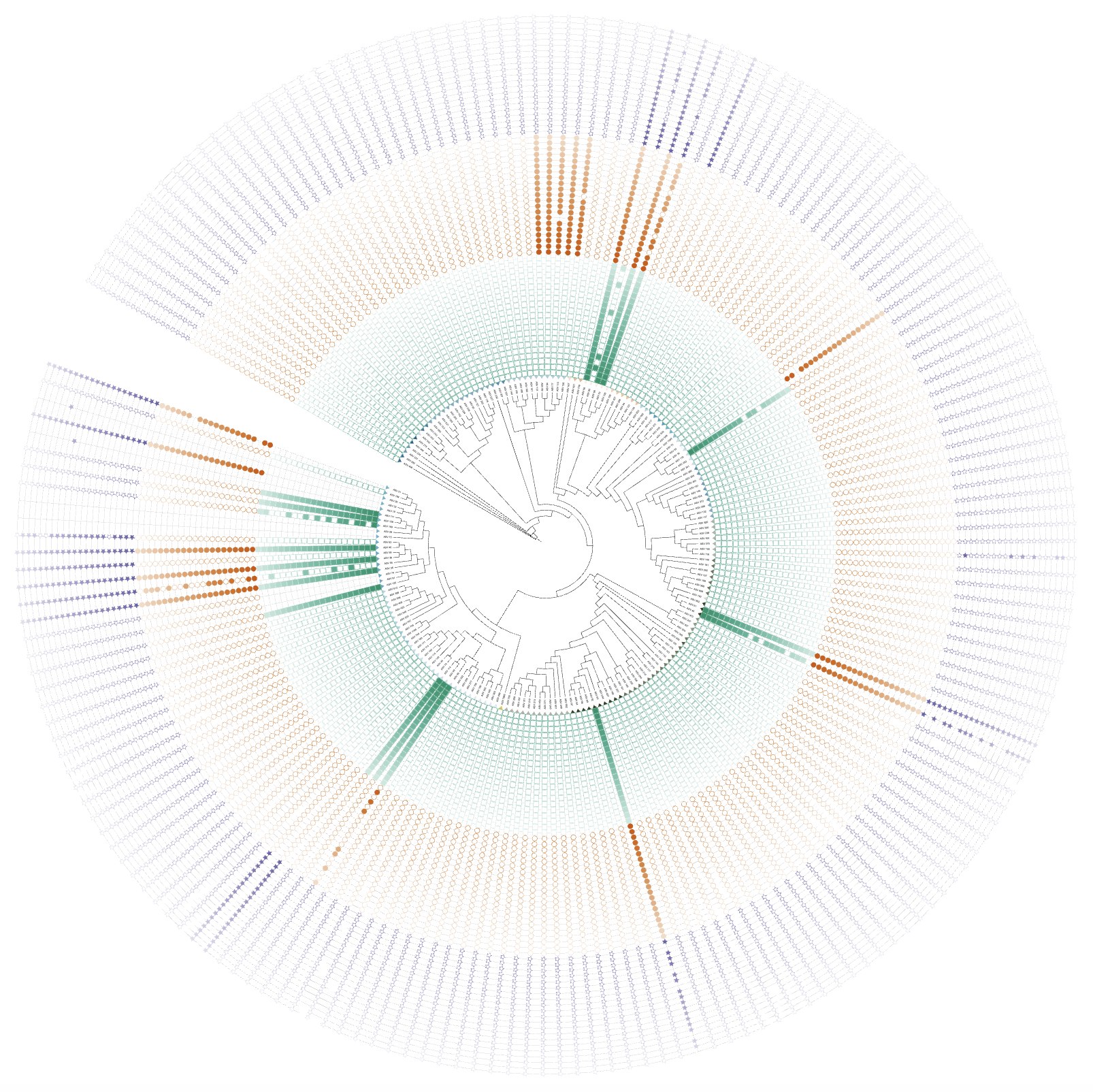

Version 1.1.11 update overview

2. Legend Order Fixes

Fixed legend ordering issues in specific dataset functions to ensure consistent behavior with user input data.

Problem Description

Previously, legends were ordered alphabetically using levels(as.factor()), causing: - Color, shape, and label orders to be inconsistent - Users could not predict final legend order - Poor user experience and confusion

Affected Functions

DATASET_COLORSTRIP: Fixed color and label order mismatch
DATASET_SYMBOL: Fixed shape, color, and label order mismatch
DATASET_DOMAINS: Fixed shape, color, and label order mismatch

Solution Implementation

All fixes use a unified approach to maintain original data frame order:

# Before (problematic code)
common_themes$legend$colors <- levels(as.factor(color))
common_themes$legend$labels <- levels(as.factor(data[[colname_data]]))

# After (fixed code)
# Get unique labels and corresponding attributes, preserving original order
unique_data <- data.frame(
  label = data[[colname_data]], 
  color = color, 
  shape = shape,  # if applicable
  stringsAsFactors = FALSE
)
unique_data <- unique_data[!duplicated(unique_data$label), ]

common_themes$legend$colors <- unique_data$color
common_themes$legend$labels <- unique_data$label
common_themes$legend$shapes <- unique_data$shape  # if applicable

Example Usage

# Load required libraries
library(itol.toolkit)
library(tibble)

# Define tree structure (example)
tree <- "((tip1,tip2),(tip3,tip4));"

# Define colors in desired order
shed_color <- tribble(
  ~Shed, ~Shed_color,
  "Farm A shed 3", "#aec7e8",    # Will appear first in legend
  "Farm A shed 6", "#1f77b4"     # Will appear second in legend
)

# Create sample data frame
df <- data.frame(
  id = c("tip1", "tip2", "tip3", "tip4"),
  Shed = c("Farm A shed 3", "Farm A shed 6", "Farm A shed 3", "Farm A shed 6")
)

# Create unit - legend order will match your data frame order
unit <- create_unit(data = df,
  key = "color_shed_colorstrip",
  type = "DATASET_COLORSTRIP",
  tree = tree)

Benefits

Consistent Ordering: Legend order now matches user-defined data frame order
User Control: Users can control legend order by arranging their data frames
Reliable Behavior: All affected functions now behave consistently
Better Alignment: Colors, shapes, and labels maintain proper correspondence

Tong Zhou

2025-09-01