v1.2.2

Overview

The itol.toolkit package version 1.2.2 continues the evolution of dual-factor coloring capabilities, extending support to additional template types and enhancing existing functionality. This version also includes important bug fixes for pie chart functionality.

Updates:

Added: DATASET_BINARY now supports third element color palette specification in dual-factor coloring.
Added: Flexible separator syntax for attribute-based dual-factor coloring - support any string as separator (single/multi-character, special regex characters).
Added: DATASET_BINARY now features flexible data conversion with a standalone convert_to_binary() function for precise control over binary data transformation.
Added: Interactive RStudio Addin binary_data_conversion provides an intuitive graphical interface for binary data conversion with real-time preview and range controls.
Added: DATASET_EXTERNALSHAPE now supports dual-factor coloring (main group + gradient) with customizable color palettes.
Fixed: DATASET_PIECHART now supports single-column data input with intelligent range detection and automatic pie segment generation.

1. DATASET_BINARY Enhanced Dual-Factor Coloring

Building upon the existing dual-factor coloring functionality in DATASET_BINARY, v1.2.2 introduces flexible separator syntax - the major innovation that allows any string to be used as a separator for grouping technical replicates. This version also adds support for specifying custom color palettes as the third element in the color parameter, and improved shape parameter control for independent shape assignment.

Available dual-factor coloring approaches:

Color-color dual-factor: color = c("main_factor", "gradient_factor") - Two color columns for dual-factor coloring
Color-color dual-factor with custom palette: color = c("main_factor", "gradient_factor", "palette_name") - Custom color palette support
Attribute-based coloring with separator: color = c("attr_name", "separator", "palette_name") - Group technical replicates by separator in column names (separator can be any string, e.g., “-”, “_“,”sample”, “_rep”, etc.)
Shape-color dual-factor: color = "gradient_factor", shape = "main_factor" - Independent shape and color control

Basic dual-factor coloring (existing functionality)

library(itol.toolkit)
library(dplyr)
library(data.table)

# Load dataset4
tree_1 <- system.file("extdata","dataset4/otus.contree",package = "itol.toolkit")
data_file_1 <- system.file("extdata","dataset4/annotation.txt",package = "itol.toolkit")
data_1 <- data.table::fread(data_file_1)

# Select data columns
# Note: Manual conversion shown here for demonstration
# In v1.2.2+, automatic conversion is available (see Section 3)
data_original <- data_1 %>% 
  select(ID, Asia, North_America, South_America) 
data_binary <- data_original %>% 
  mutate(
    Asia = case_when(
      Asia >= 1 ~ 1,
      Asia < 1 ~ 0,
      Asia == 0  ~ -1
    ),
    North_America = case_when(
      North_America >= 1 ~ 1,
      North_America < 1 ~ 0,
      North_America == 0  ~ -1
    ),
    South_America = case_when(
      South_America >= 1 ~ 1,
      South_America < 1 ~ 0,
      South_America == 0  ~ -1
    )
  )

# Create unit with single-factor coloring after manuly covert binary data
u_binary_original <- create_unit(
  data = data_binary,
  key = "BINARY_original",
  type = "DATASET_BINARY",
  color = "aaas",
  tree = tree_1
)

write_unit(u_binary_original)

# Create unit with single-factor coloring by auto covert binary data
u_binary_coverted <- create_unit(
  data = data_original,
  key = "BINARY_converted",
  type = "DATASET_BINARY",
  color = "aaas",
  method = "binary",
  tree = tree_1
)

write_unit(u_binary_coverted)

# Create unit with single-factor coloring by 2 step method covert binary data
data_binary_2steps <- convert_to_binary(
  data_original,
  negative_range = c(0, 0),
  zero_range = c(0, 1),
  positive_range = c(1, Inf),
  lower_inclusive = FALSE,
  upper_inclusive = FALSE,
  auto_detect = FALSE,
  verbose = TRUE
)

u_binary_covert_2steps <- create_unit(
  data = data_binary_2steps,
  key = "BINARY_convert_2steps",
  type = "DATASET_BINARY",
  color = "aaas",
  tree = tree_1
)

write_unit(u_binary_covert_2steps)

# Create unit with shapes
data_binary <- anno_col_group(data_binary, list(
  Asia = "Asia",
  North_America = "North_America",
  South_America = "South_America"),
  attr_name = "shape")

u_binary_shapes <- create_unit(
  data = data_binary,
  key = "BINARY_shapes",
  type = "DATASET_BINARY",
  color = "aaas",
  shape = "shape",
  tree = tree_1
)

write_unit(u_binary_shapes)

Simulated binary data demonstration with group-based shapes

# Function to generate fluctuating columns for demonstration
generate_fluctuation_columns <- function(df, base_col, num_cols, fluctuation_range, separator = "-", hierarchical = FALSE, num_samples = NULL) {
  set.seed(123)  # Ensure reproducible results
  
  if(hierarchical && !is.null(num_samples)){
    # Hierarchical naming: base_col_sample_#-rep_#
    for (sample in 1:num_samples) {
      for (rep in 1:num_cols) {
        col_name <- paste0(base_col, "_sample_", sample, separator, rep)
        df[[col_name]] <- df[[base_col]] * (1 + runif(nrow(df), -fluctuation_range, fluctuation_range))
      }
    }
  } else {
    # Simple naming: base_col-separator-#
  for (i in 1:num_cols) {
      col_name <- paste0(base_col, separator, i)
    df[[col_name]] <- df[[base_col]] * (1 + runif(nrow(df), -fluctuation_range, fluctuation_range))
    }
  }
  return(df)
}

# Prepare data for binary visualization
# Select relevant columns and generate multiple samples
data_3 <- data_1 %>% select(ID, Asia, North_America, South_America)

# Generate 4 columns for each region with ±15% fluctuation
data_3 <- generate_fluctuation_columns(data_3, "Asia", 4, 0.15)
data_3 <- generate_fluctuation_columns(data_3, "North_America", 4, 0.15)
data_3 <- generate_fluctuation_columns(data_3, "South_America", 4, 0.15)

# Round numeric values for cleaner visualization
data_3[, 2:ncol(data_3)] <- round(data_3[, 2:ncol(data_3)])


# Binary data conversion
data_3_binary <- convert_to_binary(
  data = data_3,
  force_convert = FALSE,
  verbose = TRUE,
  negative_range = c(0, 0),
  zero_range = c(0, 1),
  positive_range = c(1, 5),
  lower_inclusive = FALSE,
  upper_inclusive = TRUE,
  auto_detect = FALSE
)

# Add column group annotations using regular expressions
data_3_binary <- anno_col_group(data_3_binary, list(
  Asia = "^Asia",
  North_America = "^North_America",
  South_America = "^South_America"),
  attr_name = "color"
  )

data_3_binary <- anno_col_group(data_3_binary, list(
  s1 = "-1$",
  s2 = "-2$",
  s3 = "-3$",
  s4 = "-4$"),
  attr_name = "shape"
  )

# Create binary dataset unit with dual color and group-based shapes
# Using separator to group technical replicates
# Columns are named like "Asia-1", "Asia-2", "Asia-3", "Asia-4"
# Setting color = c("color", "-") uses prefixes before "-" as gradient groups
# All columns with same prefix (e.g., all "Asia-*") get the same gradient color
# The separator can be any string: "-", "_", "sample", "_rep", etc.
u_binary_colors_shapes <- create_unit(
  data = data_3_binary %>% select(-Asia, -North_America, -South_America),
  key = "BINARY_colors_shapes",
  type = "DATASET_BINARY",
  color = c("color", "-", "table2itol"),
  shape = "shape",  # Use group-based shape assignment
  tree = tree_1
)

write_unit(u_binary_colors_shapes)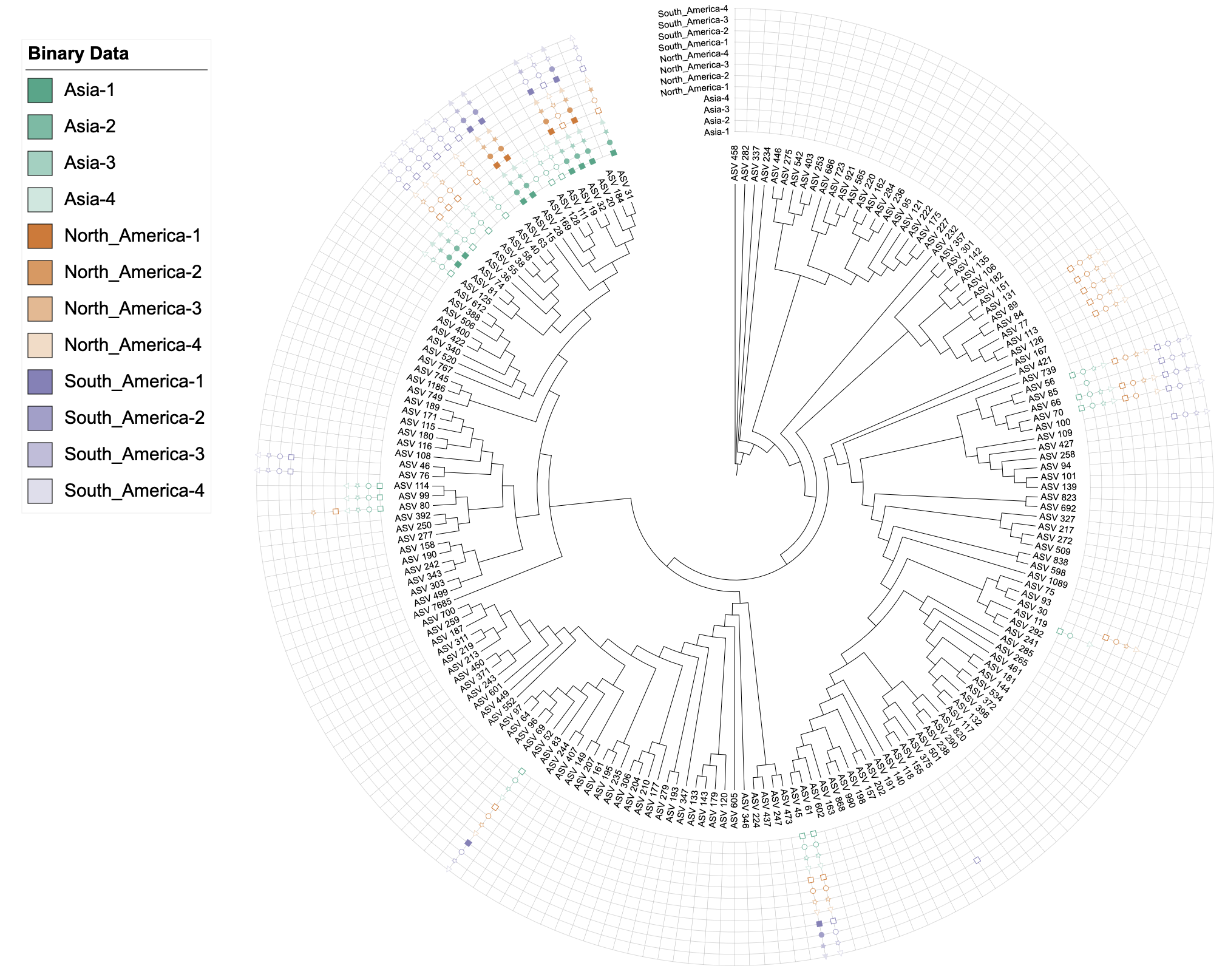

2. Flexible Separator Syntax for Attribute-Based Dual-Factor Coloring

A key innovation in v1.2.2 is the support for flexible separator syntax in attribute-based dual-factor coloring. This allows users to group technical replicates using any string as a separator in column names, providing unprecedented flexibility for data naming conventions.

Syntax: color = c("attr_name", "separator", "palette_name")

Where the second element can be any string - single character, multi-character, or even special regex characters:

Supported Separator Types

1. Single Character Separators

Dash: "-" → groups Asia-1, Asia-2 as same prefix
Underscore: "_" → groups Asia_1, Asia_2 as same prefix
Dot: "." → groups Asia.1, Asia.2 as same prefix
Any other single character

2. Multi-Character Separators

"sample" → groups Asia_sample1, Asia_sample2 as same prefix
"-rep_" → groups Asia_sample_1-rep_1, Asia_sample_1-rep_2 as same prefix
"_batch" → groups Asia_batch1, Asia_batch2 as same prefix
Any other multi-character string

3. Special Regex Characters

Automatically escaped: ., |, (, ), +, $, *, ?, [, ], {, }, ^, \
Examples: ".", "(", "$" → automatically handled by the system

# Create example data with multiple technical replicates for this section
# Technical replicates should be more similar to each other than to replicates of other regions
data_3_sep_example <- data_3 %>% select(ID, Asia, North_America, South_America)

# Generate technical replicates with hierarchical structure to demonstrate prefix grouping
# Use hierarchical naming: Asia_sample_1-rep_1, Asia_sample_1-rep_2, Asia_sample_2-rep_1, etc.
# Setting color = c("color", "-rep_") will group by prefix before "-rep_"
# All columns with same prefix (e.g., all "Asia_sample_1-rep_*") will get the same gradient color
# This demonstrates that technical replicates (rep_*) of the same sample share the same color
data_3_sep_example <- generate_fluctuation_columns(data_3_sep_example, "Asia", 3, 0.05, separator = "-rep_", hierarchical = TRUE, num_samples = 2)
data_3_sep_example <- generate_fluctuation_columns(data_3_sep_example, "North_America", 3, 0.05, separator = "-rep_", hierarchical = TRUE, num_samples = 2)
data_3_sep_example <- generate_fluctuation_columns(data_3_sep_example, "South_America", 3, 0.05, separator = "-rep_", hierarchical = TRUE, num_samples = 2)

# Binary conversion
data_3_sep_example <- convert_to_binary(
  data = data_3_sep_example,
  force_convert = FALSE,
  verbose = TRUE,
  negative_range = c(0, 0),
  zero_range = c(0, 1),
  positive_range = c(1, 5),
  lower_inclusive = FALSE,
  upper_inclusive = TRUE,
  auto_detect = FALSE
)

# Add column group annotations
data_3_sep_example <- anno_col_group(data_3_sep_example, list(
  Asia = "^Asia",
  North_America = "^North_America",
  South_America = "^South_America"),
  attr_name = "color"
  )

# Example: Multi-character separator "-rep_"
# Columns like "Asia_sample_1-rep_1", "Asia_sample_1-rep_2", "Asia_sample_2-rep_1", etc.
# Setting color = c("color", "-rep_") groups by prefix before "-rep_"
# All columns with same prefix (e.g., all "Asia_sample_1-rep_*") get the same gradient color
# This clearly shows that technical replicates (rep_1, rep_2, rep_3) share the same gradient color
u_sep_dash <- create_unit(
  data = data_3_sep_example %>% select(-Asia, -North_America, -South_America),
  key = "BINARY_sep_dash", 
  type = "DATASET_BINARY",
  color = c("color", "-rep_", "table2itol"),  # Multi-character separator
  tree = tree_1
)

write_unit(u_sep_dash)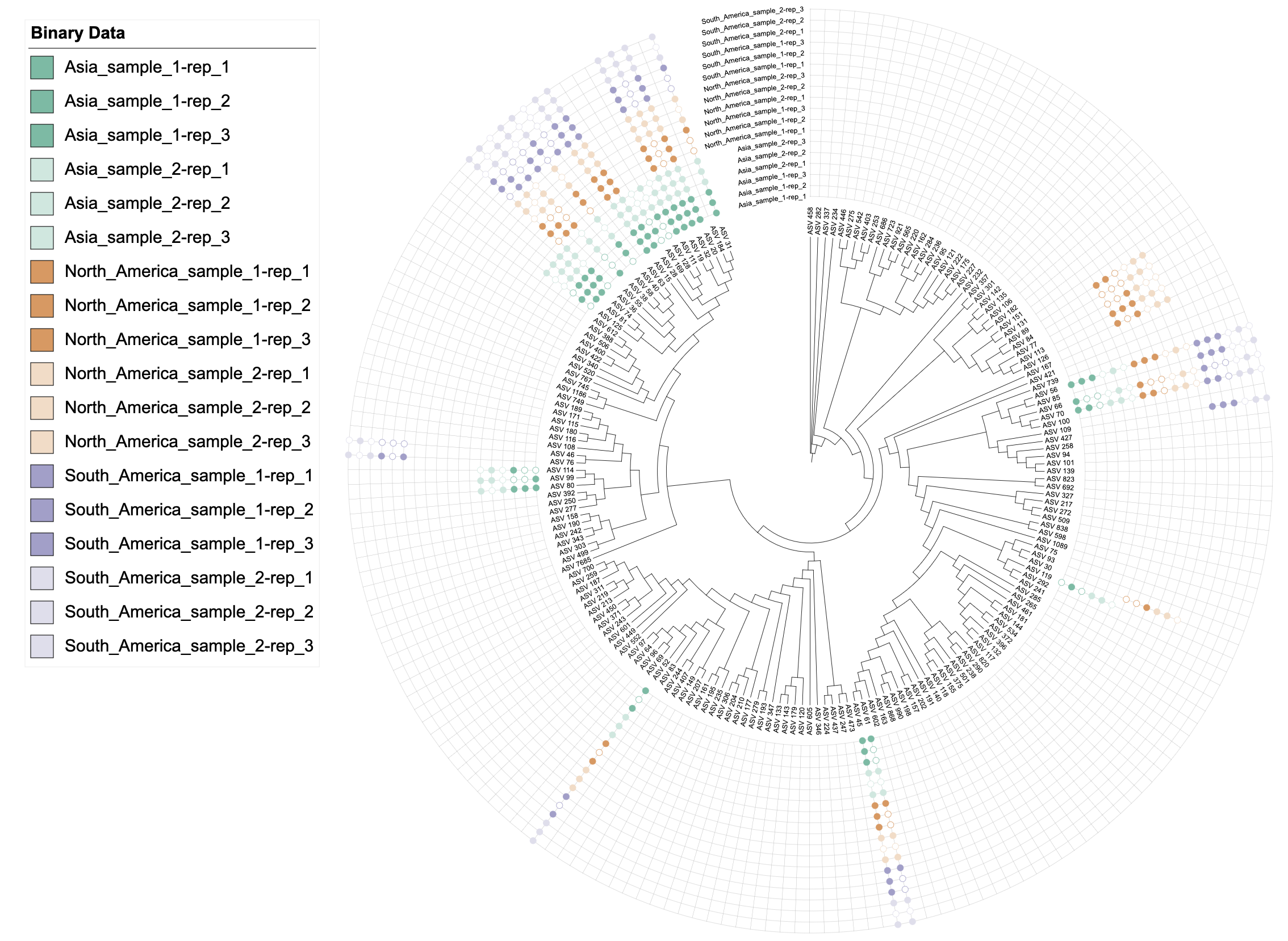

This separator syntax is particularly useful for:

Technical replicates: Group multiple technical replicates that should share the same appearance
Batch experiments: Organize data from different experimental batches
Time series: Group measurements from the same time point
Any naming convention: Adapt to your existing data naming patterns

3. DATASET_BINARY Data Conversion Enhancement

DATASET_BINARY now features flexible data conversion options. The conversion functionality has been extracted into a standalone convert_to_binary() function, providing users with more control over when and how data conversion is performed.

Two Usage Approaches

Approach 1: Automatic Conversion in `create_unit()`

Use the method = "binary" parameter to trigger automatic conversion:

# Automatic conversion during unit creation
u_auto_convert <- create_unit(
  data = data_original,  # Use data_original from example above
  key = "BINARY_auto_convert",
  type = "DATASET_BINARY",
  method = "binary",  # Enable automatic conversion
  color = "aaas",
  tree = tree_1
)

Approach 2: Manual Conversion with `convert_to_binary()`

Use the standalone function for more control:

# Manual conversion with custom parameters
data_converted <- convert_to_binary(
  data = data_original,  # Use data_original from example above
  negative_range = c(0, 0),      # [0, 0] → -1
  zero_range = c(0, 1),          # (0, 1) → 0  
  positive_range = c(1, 10),    # [1, 10] → 1
  lower_inclusive = FALSE,       # Control boundary inclusion
  upper_inclusive = FALSE,
  verbose = TRUE                 # Show conversion summary
)

# Then create unit with pre-converted data
u_manual_convert <- create_unit(
  data = data_converted,
  key = "BINARY_manual_convert",
  type = "DATASET_BINARY",
  color = "aaas",
  tree = tree_1
)

Supported Data Types and Conversion Rules

1. Proportion Data (0-1 range)

Detection: Numeric data with all values in [0, 1]
Conversion:
- 0 → -1
- < 0.5 → 0
- ≥ 0.5 → 1

2. Count/Other Non-negative Data

Detection: Numeric data with max value > 1, min value ≥ 0
Conversion:
- 0 → -1
- < 1 → 0
- ≥ 1 → 1

3. Boolean Data (Multiple Formats)

Supported formats: TRUE/FALSE, T/F, true/false, "1"/"0", yes/no
Conversion:
- TRUE/T/true/1/yes → 1
- FALSE/F/false/0/no → 0

4. Already Binary Data

Detection: Data already in {-1, 0, 1} format
Action: No conversion needed

Conversion Summary Display

The convert_to_binary() function provides detailed conversion summaries:

Converting data to binary format (-1, 0, 1)...

Conversion Summary:
         Range Values1 Values2
        <char>   <num>   <num>
1: [0, 0] → -1       1       1
2:  (0, 1) → 0       2       2
3: [1, 10] → 1       2       2

4. Interactive Binary Data Conversion Addin

Version 1.2.2 introduces a powerful RStudio Addin that provides an intuitive graphical interface for binary data conversion. The binary_data_conversion Addin allows users to visually configure conversion ranges and preview results in real-time.

Accessing the Addin

The Addin is accessible through RStudio’s Addins menu:

Location: RStudio Menu → Addins → Binary Data Conversion
Or via R console: itol.toolkit::binary_data_conversion()

Key Features

1. Dynamic Range Configuration

Three Range Sliders: Omitted (→ -1), Outline (→ 0), and Filled (→ 1)
Visual Density Plot: Shows data distribution with colored range overlays
Direct Numerical Input: Precision control with numeric input fields
Automatic Range Constraints: Zero-gap boundaries prevent overlapping ranges

2. Real-Time Preview

Data Preview: Original data with current range settings
Conversion Preview: Shows converted binary data instantly
Conversion Summary: Displays conversion statistics for each column

3. Smart Boundary Control

Lower/Upper Inclusive Checkboxes: Fine-tune range boundaries
Dynamic Labels: Range notation adapts based on inclusive/exclusive settings
- [a, b] (both inclusive)
- (a, b] (lower exclusive, upper inclusive)
- [a, b) (lower inclusive, upper exclusive)
- (a, b) (both exclusive)

Usage Example

# Access the Addin through RStudio menu
# or via R console:
itol.toolkit::binary_data_conversion()

# The Addin provides:
# 1. Dataset selection dropdown
# 2. Interactive range sliders for conversion
# 3. Real-time preview of converted data
# 4. Visual density distribution
# 5. Code generation button

Workflow

Select Dataset: Choose from available data frames in the global environment
Configure Ranges:
- Adjust sliders to define conversion ranges
- Use numeric inputs for precise values
- Set boundary inclusivity for the middle range
Preview Results:
- View original data and converted results side-by-side
- Check conversion summary statistics
- Verify data distribution visualization
Generate Code: Click “Done” to insert R code into the active script

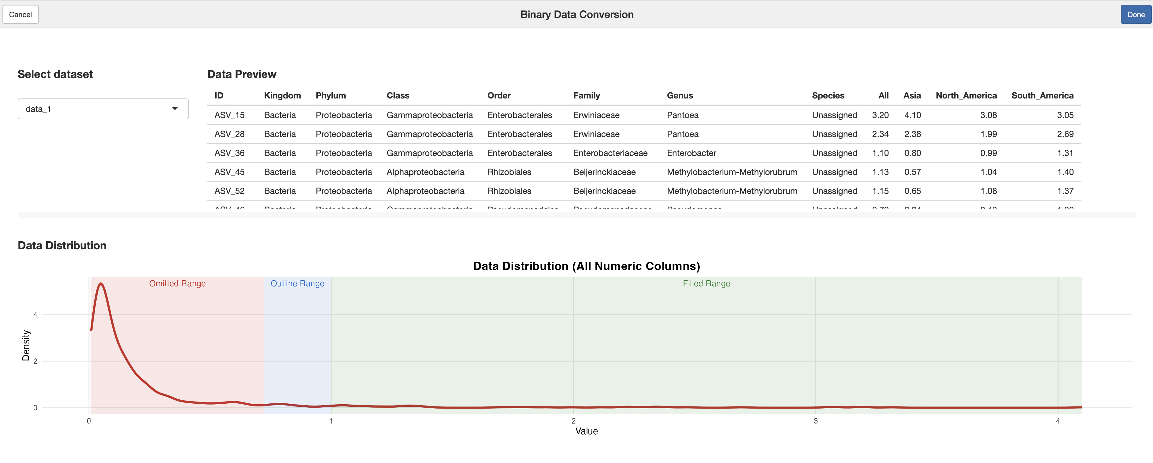
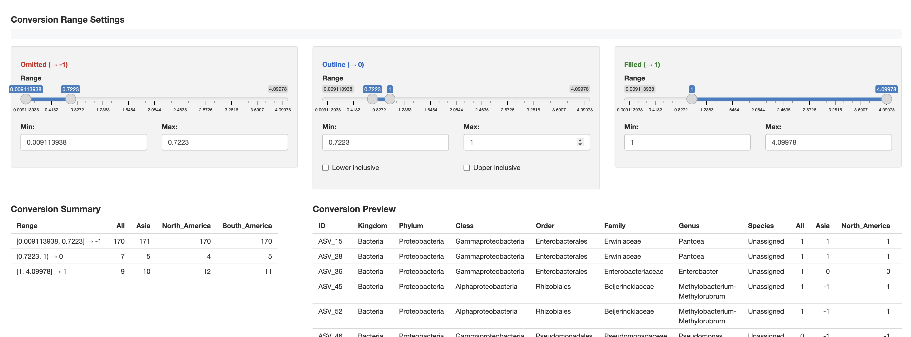
Generated Code Format

# Binary data conversion
converted_data <- convert_to_binary(
  data = your_dataset[, c("ID", "Col1", "Col2")],
  force_convert = FALSE,
  verbose = TRUE,
  negative_range = c(0.0, 0.5),
  zero_range = c(0.5, 1.0),
  positive_range = c(1.0, 4.1),
  lower_inclusive = FALSE,
  upper_inclusive = FALSE,
  auto_detect = FALSE
)

5. DATASET_EXTERNALSHAPE Dual-Factor Coloring

DATASET_EXTERNALSHAPE now supports dual-factor coloring, following the same strategy as other template types where the first factor serves as the main grouping, and the second factor creates gradients within each main group.

Single factor coloring (existing functionality)

# Add column group annotations for EXTERNALSHAPE
# Note: data_3 has columns like "Asia-1", "Asia-2", etc. (dash separator)
data_3_external <- anno_col_group(data_3, list(
  Asia = "^Asia",
  North_America = "^North_America",
  South_America = "^South_America"),
  attr_name = "color"
  )

# Single factor coloring with default palette
u_externalshape_single <- create_unit(
  data = data_3_external,
  key = "EXTERNALSHAPE_single",
  type = "DATASET_EXTERNALSHAPE",
  color = "table2itol",
  tree = tree_1
)

write_unit(u_externalshape_single)

Dual-factor coloring with separator

# Dual-factor coloring using attribute-based grouping with separator
# The separator can be any string (e.g., "-", "_", "sample", "_rep", etc.)
u_externalshape_dual <- create_unit(
  data = data_3_external %>% select(-Asia, -North_America, -South_America),
  key = "EXTERNALSHAPE_dual",
  type = "DATASET_EXTERNALSHAPE",
  color = c("color", "-", "table2itol"),  # Use "-" separator to group technical replicates
  tree = tree_1
)

write_unit(u_externalshape_dual)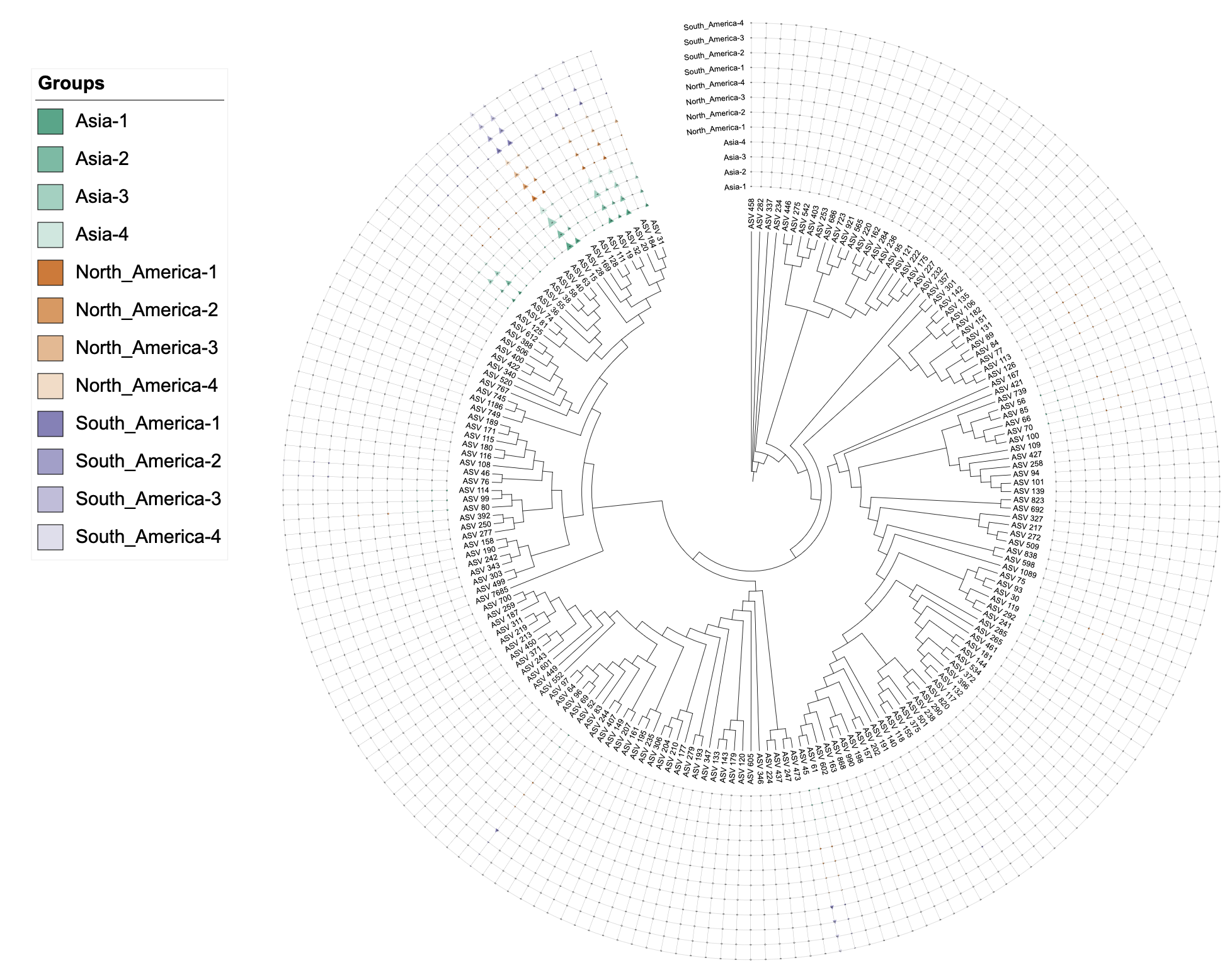

6. DATASET_PIECHART Single-Column Support

Problem Solved

Previously, DATASET_PIECHART required multiple columns to create different pie segments, causing errors when users provided single-column data (e.g., completeness percentages). The error attempt to select less than one element in integerOneIndex occurred because the color palette system expected multiple pie segments but received none.

Solution Implemented

v1.2.2 now automatically detects single-column input and creates appropriate pie segments with intelligent range detection:

Automatic Detection: When only 2 columns are provided (ID + value), the system detects this as a single-column pie chart scenario
Smart Range Detection: Automatically determines the appropriate remainder calculation based on data range:
- 0-1 range: Creates remainder as 1 - value (for proportion data)
- 0-100 range: Creates remainder as 100 - value (for percentage data)
- Other ranges: Defaults to percentage calculation 100 - value
Auto-Expansion: Creates two pie segments automatically:
- Value: The original data value
- Remainder: Calculated based on detected data range
Proper Structure: Maintains correct iTOL pie chart format with POSITION, RADIUS, and two segments
Color Handling: Ensures proper color assignment with minimum palette requirements

Usage Examples

Example 1: Percentage Data (0-100 range)

library(itol.toolkit)
library(dplyr)

# Sample completeness data as percentages
meta_CheckM <- data.frame(
  MAG = paste0("MAG_", 1:5),
  Completeness = c(85.2, 92.1, 78.5, 95.3, 88.7),  # 0-100 range
  stringsAsFactors = FALSE
)

# Create tree
tree_big <- ape::rtree(5, tip.label = meta_CheckM$MAG)

# Automatically detects 0-100 range and creates remainder as (100 - value)
unit_41 <- create_unit(
  data = meta_CheckM %>% select(MAG, Completeness),
  key = "E041_piechart_percentage",
  type = "DATASET_PIECHART",
  position = -1,
  tree = tree_big
)

write_unit(unit_41)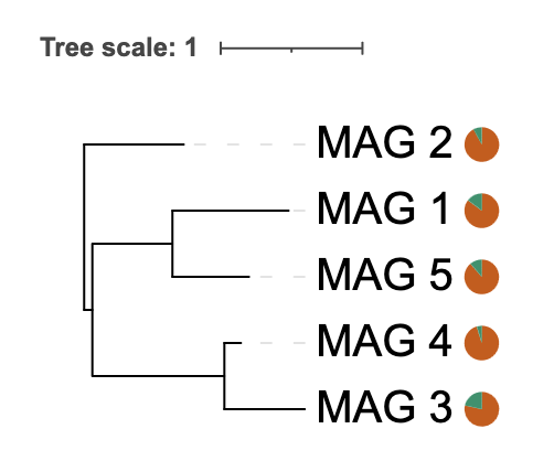

Example 2: Proportion Data (0-1 range)

# Sample completeness data as proportions
meta_CheckM_prop <- data.frame(
  MAG = paste0("MAG_", 1:5),
  Completeness = c(0.852, 0.921, 0.785, 0.953, 0.887),  # 0-1 range
  stringsAsFactors = FALSE
)

# Create tree
tree_big_prop <- ape::rtree(5, tip.label = meta_CheckM_prop$MAG)

# Automatically detects 0-1 range and creates remainder as (1 - value)
unit_41_prop <- create_unit(
  data = meta_CheckM_prop %>% select(MAG, Completeness),
  key = "E041_piechart_proportion",
  type = "DATASET_PIECHART",
  position = -1,
  tree = tree_big_prop
)

write_unit(unit_41_prop)

Output Structure

The generated pie chart will show:

Each MAG’s completeness as one colored segment
The remainder calculated based on detected data range:
- For 0-1 range: remainder = 1 - value
- For 0-100 range: remainder = 100 - value
Proper field labels: “Value” and “Remainder”
Appropriate color assignment from the default palette
Automatic range detection messages in the console

Backward Compatibility

This enhancement is fully backward compatible:

Multi-column pie charts continue to work as before
Single-column pie charts now work automatically with intelligent range detection
No changes required to existing code using multi-column pie charts
The system automatically handles both proportion (0-1) and percentage (0-100) data formats

Tong Zhou

2025-11-03

Overview

1. DATASET_BINARY Enhanced Dual-Factor Coloring

Available dual-factor coloring approaches:

Basic dual-factor coloring (existing functionality)

Simulated binary data demonstration with group-based shapes

2. Flexible Separator Syntax for Attribute-Based Dual-Factor Coloring

Supported Separator Types

3. DATASET_BINARY Data Conversion Enhancement

Two Usage Approaches

Approach 1: Automatic Conversion in `create_unit()`

Approach 2: Manual Conversion with `convert_to_binary()`

Supported Data Types and Conversion Rules

Conversion Summary Display

4. Interactive Binary Data Conversion Addin

Accessing the Addin

Key Features

1. Dynamic Range Configuration

2. Real-Time Preview

3. Smart Boundary Control

Usage Example

Workflow

Generated Code Format

5. DATASET_EXTERNALSHAPE Dual-Factor Coloring

Single factor coloring (existing functionality)

Dual-factor coloring with separator

6. DATASET_PIECHART Single-Column Support

Problem Solved

Solution Implemented

Usage Examples

Example 1: Percentage Data (0-100 range)

Example 2: Proportion Data (0-1 range)

Output Structure

Backward Compatibility

v1.2.2

Tong Zhou

2025-11-03

Overview

1. DATASET_BINARY Enhanced Dual-Factor Coloring

Available dual-factor coloring approaches:

Basic dual-factor coloring (existing functionality)

Simulated binary data demonstration with group-based shapes

2. Flexible Separator Syntax for Attribute-Based Dual-Factor Coloring

Supported Separator Types

3. DATASET_BINARY Data Conversion Enhancement

Two Usage Approaches

Approach 1: Automatic Conversion in create_unit()

Approach 2: Manual Conversion with convert_to_binary()

Supported Data Types and Conversion Rules

Conversion Summary Display

4. Interactive Binary Data Conversion Addin

Accessing the Addin

Key Features

1. Dynamic Range Configuration

2. Real-Time Preview

3. Smart Boundary Control

Usage Example

Workflow

Generated Code Format

5. DATASET_EXTERNALSHAPE Dual-Factor Coloring

Single factor coloring (existing functionality)

Dual-factor coloring with separator

6. DATASET_PIECHART Single-Column Support

Problem Solved

Solution Implemented

Usage Examples

Example 1: Percentage Data (0-100 range)

Example 2: Proportion Data (0-1 range)

Output Structure

Backward Compatibility

Approach 1: Automatic Conversion in `create_unit()`

Approach 2: Manual Conversion with `convert_to_binary()`